Measurement of a Ball Bearing
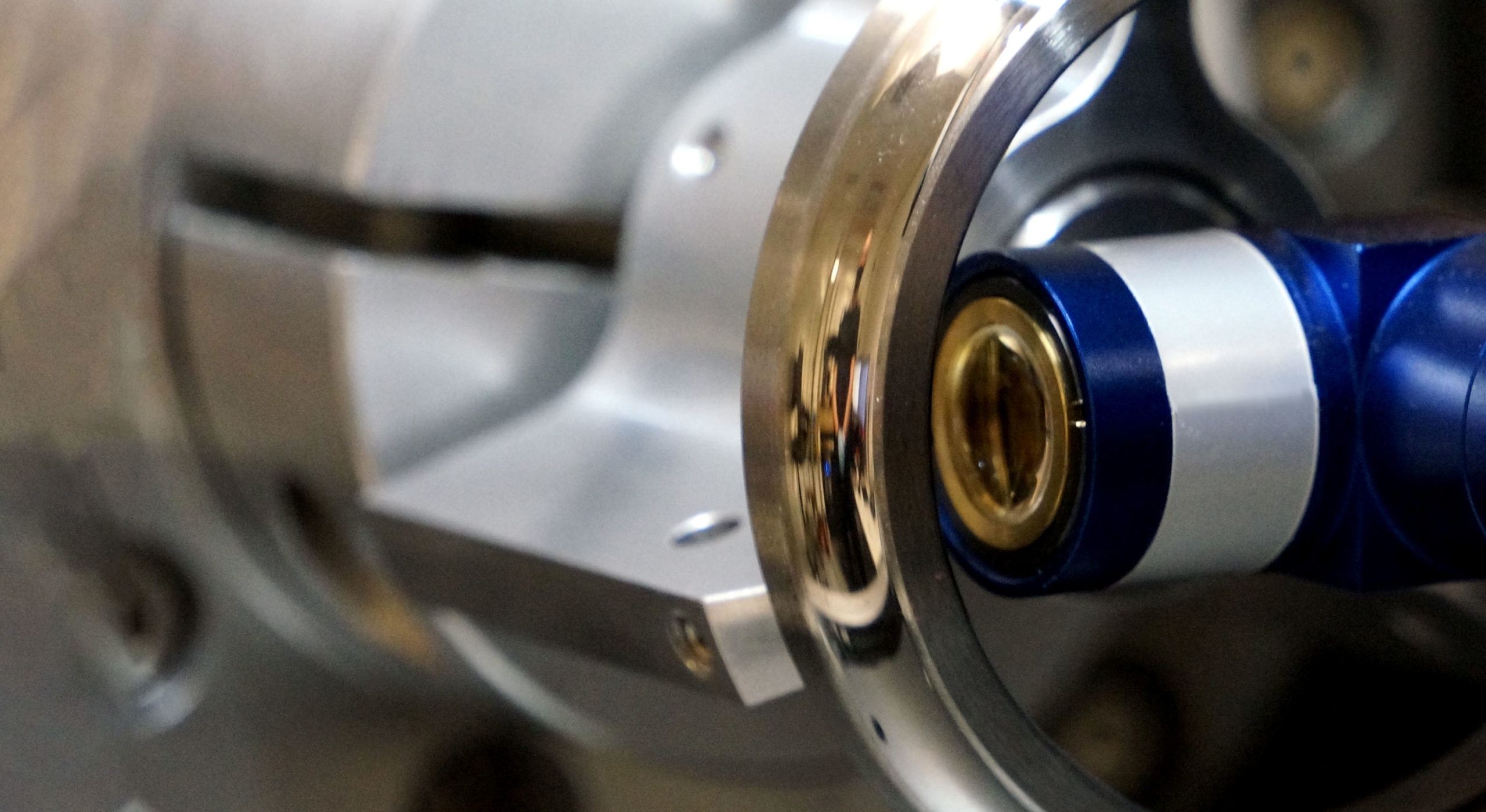
Bearings are an important part of many mechanical systems. There are several different types of bearing, an example of which, a deep groove ball bearing with a split inner race, is shown below:
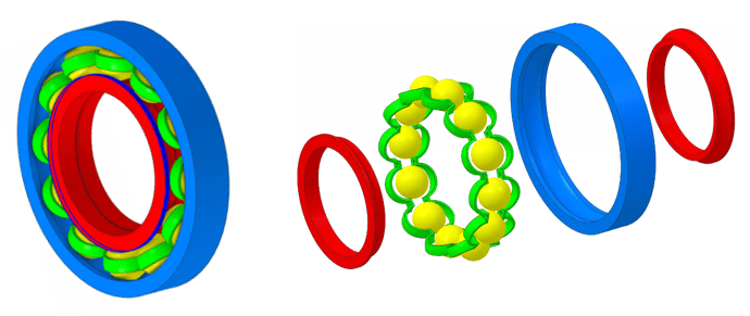
Figure 1 – The assembly of a deep groove ball bearing with a split inner race (left), with an exploded view (right). The sub-components are colour coded; in blue is the outer ring, in yellow are the spherical rollers, in green is the roller cage and in red is the inner ring, which in this case is split.
For the purposes of this document, we will be focusing on one half of the inner ring. Measurements on the outer ring are similar, albeit inverted.
What are the critical parameters for quality control on a bearing?
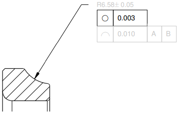
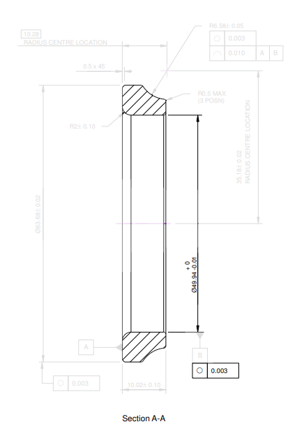
The images below show a CAD model of the inner ring.

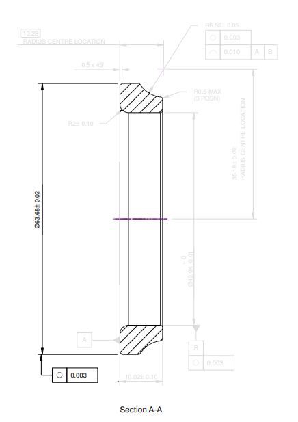
Figure 2 – a CAD model representing a typical inner bearing, with the GD&T information for this part on the right
Features that are commonly measured during quality control are found in the bearing race and the boundary dimensions of a bearing:
- Bearing race: Of main interest for the function of the bearing are the roundness and the curvature of the race relative to a theoretical radius centre location. (more …)
- Inner bore: The factors determining fit to a shaft are the roundness and the diameter. (more …)
- Outer diameter: Again, the roundness and the diameter are to be measured. (more …)
- Bearing width: In this case, the width of one of the inner rings. (more …)
These individual features will be explored in detail in subsequent sections. All measurements have been carried out with an OmniLux optical CMM, capable of measuring critical parameters on bearings with nanometre-resolution in full 3D.
Conventional measurement approaches use contact roundness machines, contour profiling machines or CMMs with a touch probe. Often, there is one specific machine for each of these measurement tasks. Scratches and other defects caused by the contacting probes or by moving the bearing from one inspection station to the next can be an issue in higher-end applications.
The OmniLux CMM can complete all measurements in a single fixturing cycle in just a few minutes without contact between the measuring probe and the bearing under inspection. This is made possible by using an optical sensor and a purpose-made 3-jaw chuck, which holds the bearing distortion-free during the measurement:
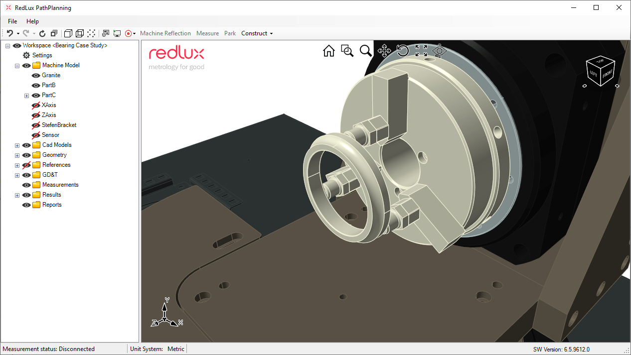
Figure 3 – A screenshot of the RedLux software, showing the CAD model of the inner bearing fixtured in the 3-jaw chuck.
Bearing race
Roundness
The roundness of the bearing raceway is typically measured by aligning the probe at the desired location on the raceway and spinning the part by a complete revolution, as shown in the image below:
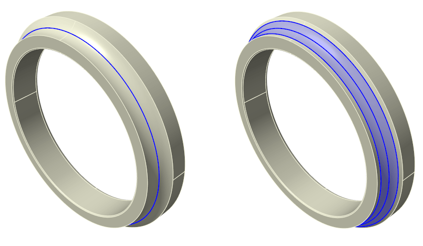
Figure 4 – Showing the concentric circle scanning strategy in blue with a single circle scan (left) and 3 circle scans (right)
Running this measurement on the OmniLux 4AB results in the data shown below

Figure 5 – Point cloud data of a single circle scan on the raceway. The colour map shows the deviation from a least squares circle fit (shown in grey). The deviation has been magnified by 4000x
The data above consists of 3600 points, with this scan taking about 3 seconds to complete.
Note the 3rd harmonic on this data – this is typical of the machining process that created this bearing.
The deviation from the circle fit extends from -0.00111 to 0.00098 mm, leading to a measured roundness value of 0.00209 um. This part is therefore within tolerance.
Curvature
The curvature of the raceway is measured by moving the probe along the part in axial direction in one or more locations, as shown in the image below.
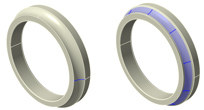
Figure 6 – Showing the axial line scanning strategy in blue with a single line scan (left) and 10 line scans (right)
This strategy can be achieved with a contour profiling machine or a RedLux OmniLux 4AB.
Running this measurement on the OmniLux 4AB results in the data shown below:
Figure 7 – Point cloud data of a single axial line scan on the raceway. The colour map shows the deviation from a segment of a least squares circle fit (shown in grey). The deviation has been magnified by 150x
The data above consists of ~13,000 points, and this scan took approximately 3.5 seconds.
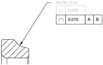
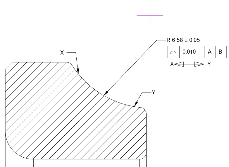
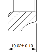
The profile exhibits a shape that is typical of bearing raceways; a more conformal region in the centre deviates further from the average curvature at the edge of the profile. Note that it is essential to have a clearly defined strategy for where the measurement will start and end; estimating a least-squares-circle (LSC) from a partial arc of such small angle is inherently uncertain, and any artefact from a fillet radius or chamfer at the edge of the race could significantly affect the fit estimate. It may be desirable on the engineering prints to include a between modifier to define the range over which the control applies, as shown below (note, the exact location of ‘X’ and ‘Y’ is not shown below for clarity, but would need to be indicated)
The deviation from the circle fit ranges from -150 nm to 88 nm, leading to a measured deviation from the intended profile of 238 nm. This part is therefore within tolerance.
One consideration with this measurement is that it only gives minimal coverage of the full surface; by luck, the 2d line profile may just hit (or just miss) a scratch, cavity or other feature, so that any two measurements may give very different results. With a measurement like this, it is always best to use multiple scans to ensure that some statistical spread is included in the data.
Surface
It can also be useful to perform full areal scans on the bearing raceway, as shown in the image below.
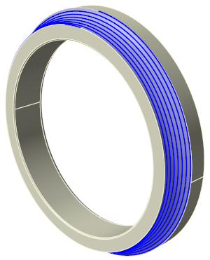
Figure 8 – Showing the spiral scanning strategy in blue, with 7 rotations
This strategy can be achieved with a traditional CMM or, much faster, with an OmniLux optical CMM. The point density using a traditional CMM will be limited to modest numbers by the scanning time, while on an optical CMM, a large number of data points can be acquired in a reasonable time. Areal scans of the raceway can be a quicker method for measuring roundness and line profile at multiple locations, as well as for analysing race height.
Running this measurement on the OmniLux 4AB results in the data shown below.
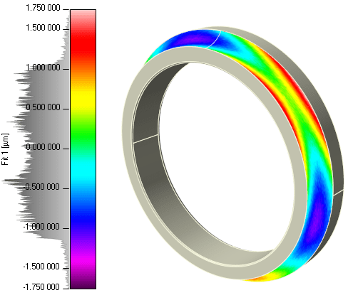
Figure 9 – Point cloud data of a spiral scan on the raceway
The data above consists of 90,000 data points and took just over 30 seconds. It gives a much better idea of what the actual shape of the bearing race looks like than a single trace can provide. Both the harmonic circumferential pattern and the above-mentioned axial pattern can be seen here in a single scan. Though not present in this case, it is not uncommon to see imperfections on the raceway surface like scratches and pits.
Inner bore
Roundness and Scale
The inner bore can be measured with similar scanning strategies to the raceway, as shown in the image below:
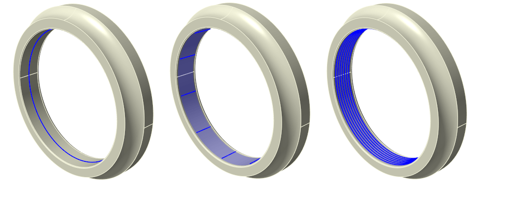
Figure 10 – Showing possible scanning strategies on the inner bore of the bearing, with a circle scan (left), axial lines (middle) and spiral scan (right)
Commonly used callouts for the inner bore are for roundness and scale (diameter). In these cases, running a circle scan is often the best option.
Running a circle scan on the OmniLux 4AB results in the data shown below:
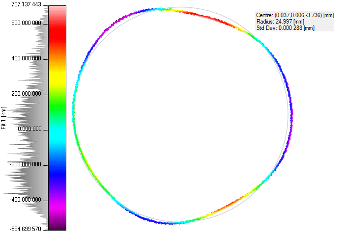
Figure 11 – Point cloud data of single circle scan on the inner bore. The colour map shows the deviation from a least squares circle fit (shown in grey). The deviation has been magnified by 2500x. Also shown in the top right are the parameters of the circle fit
This scan consists of 3600 points and took roughly 3 seconds.
The range in deviation here is 0.00127 mm. Comparing this to the roundness tolerance of 0.003 mm, this feature is within tolerance.
We can see that the fit radius of this circle is 24.997 mm, leading to a diameter of 49.994 mm. The inner diameter tolerance in this case is 50 mm +0/-0.01 mm, so this feature is also within tolerance.
Outer diameter
Roundness and Scale
The outer diameter can be measured in the same way as the inner bore.
Figure 12 – a circle scan path on the outer diameter
Running this on the OmniLux 4AB results in the following data:
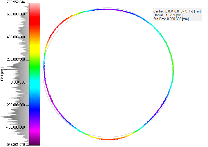
Figure 13 – point cloud data of the outer diameter. Magnification 2500x
This scan consists of 3600 points and took roughly 3 seconds.
The range in deviation here is 0.00126 mm. Comparing this to the roundness tolerance of 0.003 mm, this feature is within tolerance.
We can see that the fit radius of this circle is 31.795 mm, leading to a diameter of 63.59 mm. The inner diameter tolerance in this case is 63.68 mm +0/-0.02 mm, so this feature is out of tolerance.
Inner ring width
The width of the inner ring is calculated by measuring both the front face and the back face, and evaluating the distance between the two. These measurements can be performed using either the concentric circle scans strategy or axial line scans strategy discussed in previous sections, or by performing a full areal scan of both faces. The areal scan is advantageous as it will pick up on any local surface imperfections that the other, more limited strategies will miss.
A challenge with this feature callout is in measuring both faces in a single fixturing cycle, as one of the faces will typically be used to fixture the part during measurement. It is possible to construct a scan path that maximises coverage of the back face while avoiding the fixturing posts.
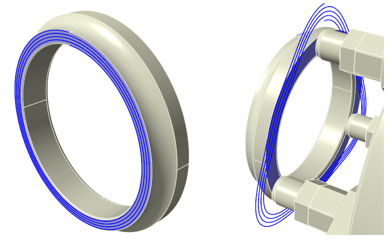
Figure 14 – Showing areal scans of the front (left) and back (right) faces to measure bearing width. The back face scan path has been adjusted to avoid the 3 fixture posts whilst still maximising surface coverage and minimising scan time
These areal scans can be performed on a traditional CMM or a RedLux OmniLux 4AB. Strategies with more limited surface coverage can be performed using manual operator measurements.
Running these measurements on the OmniLux 4AB results in the data shown in the images below.
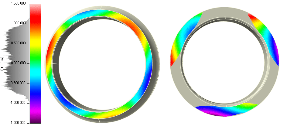
Figure 15 – Point cloud data overlaid on top of the CAD model for the inner bearing front face (left) and back face(right). A least-squares plane fit has been applied to each.
By comparing the plane fit of each face, we get a bearing width of 10.002 mm. This is well within the tolerance of 10 ± 0.1 mm.
Summary
The measurement of the bearing race, the inner and outer diameter and the width of the component have been discussed above. While these can be measured with conventional contact measurement systems, a step change in measurement speed and automation can be achieved with an OmniLux optical CMM.
Please find out more about the measurement of bearings with an OmniLux CMM here.